A Letter for Interested Students
Information for students interested in working in my group, or numerical relativity in general
Table of Contents
- Who we are and what we do
- Gravity takes on a life of its own
- Thick disks and hypermassive stars
- Turbulence and the great paradoxes of fluid dynamics
Who we are and what we do
Hello! I’m pleased that you’re interested in the work going on in the WSU numerical relativity (NR) group. It’s a good idea for any student to investigate many research fields and groups. Numerical relativists smash neutron stars and/or black holes into each other in computer simulations to see what happens. For many of us working in the field, this is intrinsically fun enough to demand no further justification, but NR simulations do have scientific value for two fields. First, they contribute to gravitational physics, the study of strongly curved spacetimes. Black holes and neutron stars are the best laboratories for studying extreme gravity and testing general relativity that nature has provided us. Second, they contribute to multimessenger astronomy, the study of violent phenomena in the universe that can be observed using different types of signals, as opposed to just different wavelengths of electromagnetic radiation. The events we model are detectable both electromagnetically and via gravitational waves, and models are needed to make sense of the observations. The application to gravitational physics justifies our (fairly steady) funding from NSF, and the application to multimessenger astronomy justifies our (intermittent but very helpful) funding from NASA. Most of this money goes toward supporting graduate students; we’re grateful to these agencies and to the taxpayers.
The NR group at WSU is led by me, Prof. Matt Duez. It is part of the “Simulating eXtreme Spacetimes” (SXS) collaboration, that includes multiple academic institutions, united by our common code. There is also another relativity group at WSU, led by Prof. Sukanta Bose and more directly connected to LIGO-Virgo, which I also encourage you to check out.
Now for more detail on the physics we work with.
Gravity takes on a life of its own
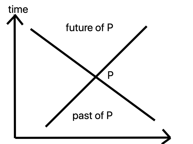
Light cones and the meaning of temporal order
Consider for a moment the momentous consequences of the fact that nothing can travel faster than the speed of light. Imagine an event, a particular place at a particular time (something like “the fall of the Bastille”). Call it P. We can mark it on a spacetime diagram, with time chosen to be the vertical axis. Events are points on such a diagram. Light rays are 45 degree lines. The possible light rays (the light cone) passing through P divide all of spacetime into three regions. Above is the future of P. A signal or object traveling at less than the speed of light can go from P to any of these events. These events can be affected by what happened a P; participants at those events might remember P. Below is the past of P. Signals and objects moving at less than the speed of light can go from these events to P. What happens at P is affected by them. These relations of influence and memory, of cause and affect, are what we mean by “past” and “future”. Time simply is the order of causality. If this is so, then the other events, not connectable to P by a physically traversable path, are neither in P’s past nor in its future. They have no causal, hence no temporal, relation to it. Indeed, different global Lorentz frames will disagree about whether P or any of these other events happen first.
When we think of gravity, we usually think of it as the pull of one object on another. The sun pulls on the Earth (and vice versa), etc. From introductory physics classes, we know there is another way of thinking of it. Rather than saying that the sun pulls on the Earth, we can say that the sun creates a gravitational field, and the gravitational field at our location is what pulls on the Earth. For weak-gravity, slow-moving systems like the solar system, this complication may seem unimportant, even pedantic. The sun makes a radial field pulling everything toward it; why not just say the sun pulls everything toward it?
Well, if there is fast motion or strong gravity, the difference becomes very interesting. Does the sun’s gravitational field at Earth’s location point toward where the sun is right now? From what we said above, one can’t really say what event on the sun’s path through spacetime corresponds to “right now” on Earth. If nobody’s moving relativistically, we can define an approximate global Lorentz frame to give “right now” a meaning (although one that the laws of physics don’t care about). Even so, if no signal can travel faster than light, the field here can at best be affected by where the sun was a light-travel time (8 minutes) ago. We are pulled not toward where the sun is, but toward where it was.
Gravitational waves
o far, there’s nothing special about gravity. You remember that electromagnetic fields also depend on charges and currents at retarded times. You’ll also remember that if the charges and currents are accelerating, electromagnetic waves are produced. These waves are much longer-ranged than static fields. The electric field of a static charge goes like \(1/r^2\), but that of a radially outgoing EM wave falls off like \(1/r\). (The energy flux, which goes like \(E\times B\), falls off like \(1/r^2\).) Once generated, EM waves require no further help from charges and currents; they continue traveling through space forever. In fact, there are perfectly good solutions of Maxwell’s equations with nothing but EM waves (no charges or currents anywhere at any time). With Maxwell’s completion of the theory of electromagnetism and discovery of EM waves, the electromagnetic field could be seen to have a dynamics, a “life”, all of its own. In any causal theory of gravity, including general relativity, gravity will likewise take on a life of its own, and there will be gravitational waves which will fall off like \(1/r\) and be detectable much further away than we could ever hope to feel the source’s gravitational pull.
Electric charges and currents act as sources for electromagnetic fields. Mass and mass currents acts as sources for spacetime curvature. Gravitational waves are vacuum (i.e. source-free) solutions of Einstein’s field equations, just as electromagnetic waves are vacuum (source-free) solutions of Maxwell’s equations. Although neither type of wave needs sources to continue in existence and propagate, sources are important for generating these waves. A time-varying electric dipole generates an electromagnetic wave; a time-varying mass quadrupole generates a gravitational wave. Remember, this is what dipoles and quadrupoles look like:
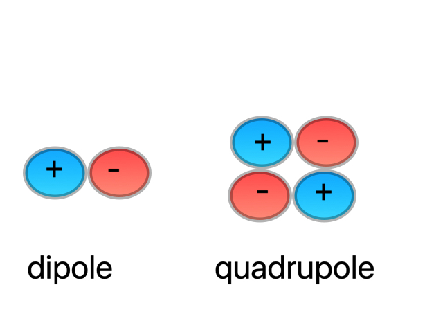
(Density is always positive, so there are no mass dipoles.) More precisely, the quadrupole moment is quantified by the quadrupole moment tensor
\[\int \rho(x_i x_j - \frac{1}{3}\delta_{ij}r^2) d^3x\]and the gravitational wave spacetime distortion depends on time derivatives of this.
One mass distribution with a strong quadrupole component would be two blobs of matter on either side of the origin, so you won’t be surprised that binary systems make the best gravitational wave sources, with the time-dependence supplied by the motion of the two objects orbiting each other.
Black holes
Strong gravity allows gravity to take on a life of its own in an even more shocking and menacing way. If gravity is really spacetime curvature, then it can influence light cones and, in extreme cases, tip them over, like this:
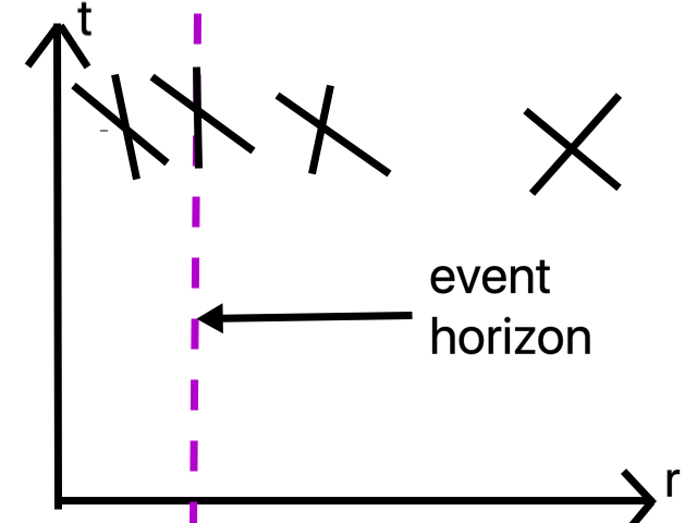
Of course, I’ve had to suppress two dimensions, so this is only showing time and a radial variable; all of the light rays shown are radial, traveling directly towards or away from the origin. (Remember, on a spacetime diagram, the origin appears as the vertical axis.) All observers must travel within their light cones, and all signals of any sort must travel in or on their light cones, so you can see that it’s impossible for any sort of signal to leave the region to the left of the purple dotted line. Things and information can go in, but they can’t go out. The dotted line is an event horizon, and inside of it is a black hole.
Our Newtonian intuition is that when things fall into a black hole, the black hole is pulling them in, but that can’t be right at all. There can be no communication of any kind from the black hole to the outside—for that to happen, a signal would have to break out of its own light cone. The interior of the black hole is inaccessible in exactly the same way as the future is inaccessible to the past. Using light cones to define “past” and “future”—as one should—we see that no event inside the black hole is in the past of any event outside. The matter that collapsed to form the black hole might have vanished without a trace, and we outside observers could be none the wiser.
So what pulls an object toward the black hole? It can only be the gravitational field—actually, the spacetime curvature—at the location of the object. And what makes the spacetime have that curvature at the object’s location? Once again, it can’t be anything inside the black hole. In fact, no matter needs to be involved at all. The spacetime curvature of a black hole can maintain itself. It’s the most dramatic case one could imagine of spacetime curvature driven by its own dynamics.
But what if I just look at a black hole. Won’t I see something?
Remember, what you see when you look in a particular direction isn’t necessarily what is there in that direction, just what light is hitting your eye coming from that direction. Given some light sources near a black hole, one can trace the paths of light rays through the curved spacetime to determine what an observer at some location would see. Often there is a “shadow” range of directions in which a close observer would see black. This means that no light is coming to your eyes from these directions.
What if I stick my hand inside the horizon to feel what’s going on inside?
This is not recommended. To stay in one piece, the rest of you will be crossing inside soon afterward. On the bright side, your hand that crosses the horizon first won’t go numb–by the time nerve signals from your hand reach your head, your head will be inside the horizon. As a matter of fact, you won’t even know when you’ve crossed the horizon. It’s empty space and locally won’t seem in any way special. From the perspective of an observer right at the horizon, the horizon is moving outward at the speed of light, and the observer would need to move at the speed of light just to keep up. (This can be seen by looking at the light cones above.)
What equations go into a numerical relativity simulation
Let’s take a sample system: the merger of a black hole with a neutron star. This problem has a lot of ingredients. There is a fluid star. There is a black hole. As the two move, they give off gravitational waves.
First, consider how one would simulate this system on a computer using Newtonian physics. The neutron star is a fluid, so at each point it can be described by its density \(\rho\), internal energy density \(U\), and velocity \(\vec{v}\). These obey the equations of hydrodynamics:
\[\frac{\partial\rho}{\partial t} + \nabla\cdot(\rho v) = 0\] \[\frac{\partial}{\partial t}(\rho v^i) + \frac{\partial}{\partial x^j}(\rho v^i v^j + P\delta^{ij}) = \rho g^i\] \[\frac{\partial}{\partial t}\left(\frac{1}{2}\rho v^2 + U\right) + \nabla\cdot\left[\left(\frac{1}{2}\rho v^2 + U + P\right)\right] = \rho g\cdot v\]where \(P\) is the pressure and \(\vec{g}=-\vec{\nabla}\phi\) is the gravitational acceleration. These equations are just the laws of conservation of mass, momentum, and energy, respectively. The first, for example, just says, in the language of a partial differential equation, that the mass in a region only changes because of the flux of mass in and out through the region’s boundary. To complete the description of the fluid, one must specify an equation of state, a rule for computing the pressure, e.g. a function \(P=P(\rho,U)\).
In a Newtonian simulation, the black hole is a point mass. It has mass \(M_{\rm BH}\) and position \(\vec{x}_{\rm BH}\). If we like, we can set by hand a “horizon radius” and arrange that any fluid matter inside this distance from the point mass is removed from the simulation, with its mass and momentum incorporated into the point mass. The “black hole” will have its own equation of motion \(M_{\rm BH} \ddot {\vec{x}}_{\rm BH} = \ldots\) which makes the point mass’s momentum change because of forces from the fluid and momentum of matter that has “fallen in”.
The gravitational potential will come from the black hole and the neutron star:
\(\nabla^2\phi = 4 \pi G [\rho + M_{\rm BH} \delta(\vec{x}-\vec{x}_{\rm BH})]\).
Gravitational waves don’t exist in Newtonian physics, but one can do an integral to get the quadrupole moment, measure its time-dependence, and estimate the gravitational wave signal from that.
Having thought through the Newtonian way, you are now ready to appreciate how different things are in general relativity. First, we’ll consider the evolution of the neutron star fluid. That actually isn’t much different. One still evolves the same conservation laws of mass, momentum, and energy. They look almost like their Newtonian equivalents, and the differences aren’t interesting. The big difference is in the other stuff.
In Newtonian physics, gravity is a force caused by the field \(\phi\). In GR, there is no gravitational force; there is only curvature in the geometry. The equivalent of \(\phi\) is the spacetime metric tensor g. Recall that the metric tensor tells you how to measure the proper distance between nearby points. In Newtonian physics, with the usual Cartesian coordinates, this is just the Pythagorean theorem:
\[\Delta s^2 = \Delta x^2 + \Delta y^2 + \Delta z^2\]In special relativity, time and space intervals depend on the observing frame (“time dilation”, “length contraction”), but there is a combination which is an invariant separation between events:
\[\Delta s^2 = -c^2\Delta t^2 + \Delta x^2 + \Delta y^2 + \Delta z^2\]In the presence of curvilinear coordinates and/or curvature, the equation will be more general. For a general coordinate system, let us label our coordinates generically as (\(x^0\),\(x^1\),\(x^2\),\(x^3\)). Note that there are four of them because spacetime is 4D; one will usually be a time coordinate. The proper distance will still depend on quadratic combinations of the coordinate intervals \(\Delta x^a\), but there may be a coefficient in front of each term, and each coefficient can be a function of space and time.
\[\Delta s^2 = g_{ab}\Delta x^a\Delta x^b = g_{00}\Delta x^0\Delta x^0 + g_{01}\Delta x^0\Delta x^1 + \ldots + g_{22}\Delta x^2\Delta x^2\]The metric components \(g_{ab}\) contain all the information about the spacetime. In particular, they provide the light cones, which are the null paths for which \(\Delta s^2 = 0\). They have their own equations of motion, which are partial differential equations and are in fact fairly similar to wave equations
\[\left(\frac{\partial^2}{\partial t^2} - \nabla^2\right) g_{ab} \sim 16\pi T_{ab}\]\(T_{ab}\), the stress-energy tensor, contains information about the mass, energy, and momentum, which serve as sources of the spacetime curvature. I put the \(\sim\) sign because the above isn’t exactly right. The full Einstein field equations are a bit more complicated; they have nonlinear terms which made it difficult to figure out how to evolve them stably. Those problems are solved now, though, so we needn’t bother about the nonlinear terms; they must be added, but they don’t change the general picture of what goes into these simulations.
We still have to add the black hole and the gravitational waves, right? Nope. We’re done. All of that is contained in the metric tensor. Black holes and gravitational waves are just aspects of spacetime curvature. Just setting \(g_{ab}\) appropriately makes there be a black hole; just evolving \(g_{ab}\) according to its field equations makes the black hole move and grow appropriately. Waves of \(g_{ab}\) propagating out to the outer boundaries just are gravitational waves.
That’s what goes into a numerical relativity simulation.
Thick disks and hypermassive stars
Neutron stars and their binaries
Nearly all the NR work at WSU involves neutron stars in one way or another. Neutron stars are fascinating objects, made of the densest known form of matter in the universe. You know that in ordinary matter, nearly all of the mass is concentrated in the atomic nuclei, which take up a very small fraction of volume. For an atom, the nucleus takes up \(\sim 10^{-15}\) of the volume. The nuclei themselves are incredibly dense, around \(10^{15}\) g cm\({}^3\). The interior of neutron stars is nuclear matter, meaning it is the density of nuclei—no empty space in between. One can imagine it as what would happen if the atomic nuclei in atoms were to be brought so close together that they touched and dissolved into a single gigantic nucleus. A typical neutron star has a mass a little more than that of the sun and a radius of around a dozen kilometers (an oddly humanly comprehensible scale for an astronomical object). It’s a city-sized atomic nucleus.
Besides their high compaction, the important thing to know about neutron stars is that they are degenerate objects, meaning that the pressure that holds them up against their own gravity is not thermal pressure. It is pressure that would be there even if the temperature were absolute zero. The sources of pressure in neutron star matter are 1) nuclear forces, which can become repulsive if particles get too close together, and 2) kinetic energy that particles are forced to have just because of the Pauli Exclusion Principle even in the absence of thermal energy. Because the effect of nonzero temperature is usually so small, neutron stars can usually be treated as “cold” objects, even when their temperature is billions of degrees.
Two neutron stars caught in each other’s gravity will also form a binary system, will also emit gravitational waves that slowly extract orbital energy, will thus slowly spiral toward each other and eventually merge. When two neutron stars merge, one would expect the result to be a more massive neutron star—after all, the nuclear density matter from the two neutron stars goes into this post-merger blob, and what else would one call something made out of that stuff? However, it turns out that there is an upper limit to the mass that a neutron star can have, and adding the masses of two ordinary neutron stars may well put one over that limit.
Mass limits and stability
To persist more than a very short time, a neutron star (or any other star) must be in an equilibrium state. That is, the net force on each parcel of fluid in the star must be zero. For a nonspinning star, the only forces are (to think in a Newtonian way for a moment) gravity (pulling fluid elements together) and pressure (pushing them apart), so these must exactly balance each other everywhere in the star. Much of the theory of neutron stars involves building equilibrium models. Usually it is acceptable to ignore spin and to ignore heat (i.e. take the neutron star to be completely degenerate). Then, one can find an equilibrium density profile for each choice of central density \(\rho_c\). If one does this for a neutron star-like equation of state, one finds something like the following:
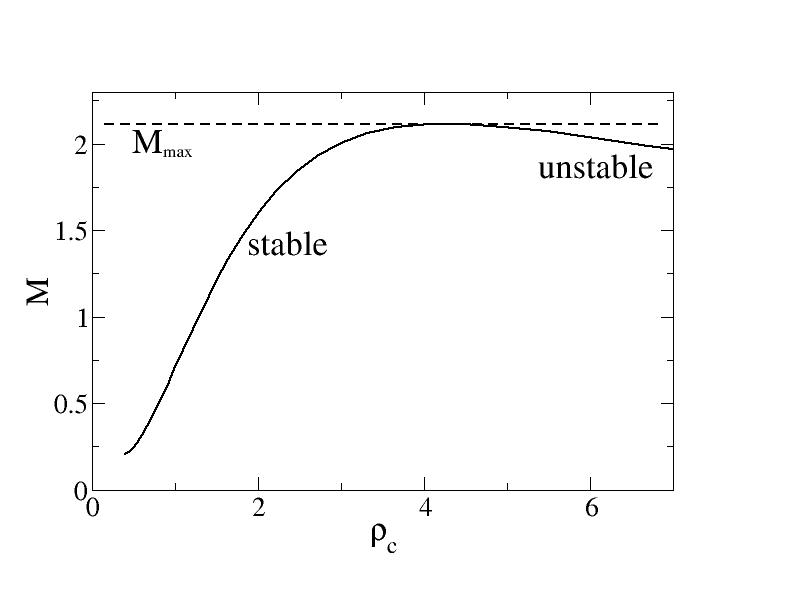
Interestingly, one cannot make equilibria beyond a maximum mass \(M_{\rm max}\); they just don’t exist. There appear to be two equilibrium central densities for each mass. However, only one could be found in the real universe. Remember, not all equilibria are stable. A system at an unstable equilibrium point will move away from the equilibrium if perturbed. One can make a model of this by plotting the strength of gravity and pressure as functions of radius \(R\) for a configuration of fixed mass. (As an aspiring physicist, you should actually try this. Use total energy as a proxy for strength. \(E_G\sim GM^2/R\), \(E_P\sim PV\), then assume an equation of state \(P\propto V^{-\Gamma}\) and see how your results depend on your choice of exponent \(\Gamma\).)
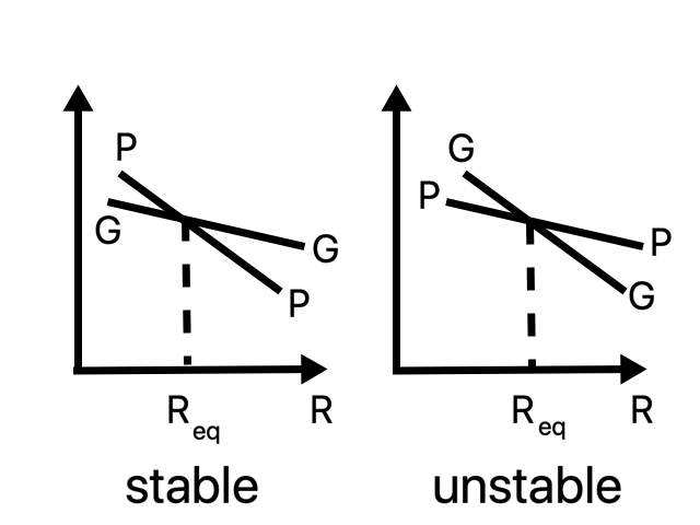
At equilibrium \(R_{\rm eq}\), the forces balance. In a stable equilibrium, pressure should “win” if the star is contracted to \(R<R_{\rm eq}\), and gravity should “win” if the star is expanded to \(R>R_{\rm eq}\); that way, force imbalance will tend to move the star back to equilibrium. For this, we need pressure to depend more steeply on \(R\). The equilibria at densities higher than that of the maximum mass turn out to have the opposite, unstable, arrangement. If one evolves such a star on an NR code, it will either expand to oscillate about the stable equilibrium at that mass, or it will collapse to a black hole.
Is there any way to get around the maximum mass? Let us try relaxing our assumptions. Binary neutron star merger remnants are very hot (\(T>10^{11}\)K) and thus not entirely degenerate. This means that there is thermal pressure to help hold the star up against its own gravity. Maybe that will help. There is also spin. When two neutron stars merge, their orbital angular momentum is transferred to spin angular momentum of the remnant, so remnants can spin at something like a thousand times per second. This provides a centrifugal force support against gravity. NR simulations have investigated both thermal and rotational support and find that one can indeed use them to make objects with \(M>M_{\rm max}\) which don’t immediately collapse.
However, introducing spin makes stars subject to other types of instabilities. According to binary neutron star merger simulations, remnants are not only spinning rapidly; they are also spinning differentially, that is, with different angular velocity \(\Omega\) in different parts of the remnant. \(\Omega\) is highest in a ring in the interior and falls off toward the surface. Let us call this function \(\Omega(r)\) the rotation profile. Flows of this sort, with \(d\Omega/dr<0\) are known to be unstable to the magnetorotational instability (MRI). As one might guess from its name, the MRI is triggered by a weak magnetic field inside the flow coupling fluid elements rotating at different rates. Unlike the instability we considered earlier for stars with high \(\rho_c\), the MRI don’t cause a star to collapse or expand as a whole. The unstable, exponentially growing modes tend to be much smaller than the star, with wavelength of order \(\lambda_{\rm MRI}\sim v_A/\Omega \sim B/(\sqrt{\rho}\Omega)\), where the Alfven speed \(v_A\) is a characteristic speed associated with waves of plucked magnetic field lines. The effect of the MRI will thus be to cause churning of the fluid on small scales, which will develop into turbulence. The overall density and rotation profiles of the remnant won’t be affected at first. Over longer periods of time, turbulence will have a profound effect on the rotation profile.
Dynamical vs secular evolution
At this point, I would expect you, as an aspiring physicist, to have a question. What exactly do I mean by “at first” and “over longer periods of time”. How long is “long”? This is a question of timescales, one of the astrophysicist’s greatest tools.
If the remnant weren’t in equilibrium at all, how long would it take for the force imbalance to result in a large change, e.g. for it to collapse to a black hole? This is the dynamical timescale. One might expect it to depend on \(M\), \(R\), and \(G\). You can convince yourself that there is only one combination with units of time, the free-fall timescale: \(\tau_{\rm dyn} \sim \tau_{\rm ff} \sim \sqrt(\frac{R^3}{GM})\). (Not coincidentally, this should remind you of Kepler’s third law. Planets orbit on the same timescale that they “fall”.) A configuration like the high-density equilibria above that has a large-scale dynamical instability will not last beyond durations of order \(\tau_{\rm dyn}\)
Other effects act on longer timescales. For example, the heat in a merger remnant certainly won’t last forever; it will be radiated away by neutrinos in a matter of seconds. Since this is much longer than the dynamical timescale, the star can continually adjust to the cooling, proceeding from one equilibrium to another. At any given time, the star is close to dynamical equilibrium, but the equilibrium configuration slowly changes; we can call this “secular evolution”.
What about the rotation support? Initially after merger, some angular momentum will be carried away by gravitational waves. Even after these cease, angular momentum might be drained by winds of outgoing matter. Furthermore, turbulence driven by the MRI will tend to transport angular momentum outward, causing some regions to slow down and others to speed up. This is another secular effect (the effect on the rotation profile, that is; the MRI itself is a dynamical instability), and will alter the rotation support on a secular timescale. Once again, we can think of the remnant as evolving from the dynamical equilibrium of one rotation profile to the dynamical equilibrium of another. Ultimately, the remnant can only settle down when it achieves rigid rotation or reaches a configuration that is dynamically unstable and collapses to a black hole.
Categories of astrophysical equilibria
One way of thinking about the role of numerical relativity is that we are providing support to gravitational wave observatories by modeling their sources and providing waveform predictions that are more accurate than other methods can provide. I don’t want to be dismissive of this understanding, which motivates most of NR funding. However, NR is also more generally a tool for studying the possibilities of relativistic equilibria. Our simulations can distinguish dynamically stable from unstable configurations. For stable configurations, we can follow the secular evolution driven by radiation and turbulence, tracking the system from equilibrium to equilibrium until we reach a secular equilibrium or a dynamical instability. If instability and dynamical collapse are found, we can explore the outcome of the collapse. Is it an isolated black hole, or is it surrounded by an accretion disk? How big is the disk? Continuing the simulation would then reveal the secular evolution of the disk.
Turbulence and the great paradoxes of fluid dynamics
The surprising difficulty of falling into a black hole
It may sound strange, but it’s true, and I always enjoy pointing it out to students: it’s actually very hard to fall into a black hole. I mean, if I had you a rock and tell you to throw it so that it falls into a black hole—let’s say that the black hole is much closer than any other astronomical body, but that for safety your distance from the black hole is much farther than the horizon radius—you will probably fail. The reason comes down to first-year undergraduate physics. Unless your aim is very good, you’ll impart some angular momentum \(L = m r \times v\) onto the rock relative to the black hole. Since the rock experiences no torque as it flies toward the black hole, its angular momentum will be conserved. As it gets closer to the black hole, angular momentum conservation will force its orbital speed to increase. Eventually, centrifugal force will overcome gravity, and the rock will start being pushed away from the black hole, settling on an at-first nearly parabolic trajectory. (You’re not that strong, and you threw the rock from far away, so its orbital energy is close to zero compared to \(GM/r_{\rm BH}\).) Of course, the same considerations apply to throwing rocks at objects other than black holes. Throwing a rock onto the sun, for example, takes some doing. owever, throwing a rock into the sun is still much easier than throwing a rock into a black hole of the same mass. This is because the sun is much less compact. One doesn’t have to lose nearly as much angular momentum to hit the surface of the sun as one would have to lose to reach the event horizon of a black hole of the same mass.
Now, we often find analogous cases in nature where gas is sucked in by a black hole’s gravity, say from a binary companion star. It has angular momentum, so it can’t just fall in. Parcels of gas will push on each other until the gas settles into orderly circular orbit, with each parcel orbiting at a rate given by Kepler’s third law, as if each bit of gas was a planet orbiting its star. The gas forms a disk. Now, it seems that conservation of angular momentum will keep the gas orbiting there forever. And yet, we have observational evidence that gas does fall in toward and into the black hole—accretion happens. But how is this possible?
Angular momentum can’t disappear, so it must be transferred. A parcel of gas can lose its angular momentum and move inward if it can pass off this angular momentum to another parcel of gas, whose orbit will then move outward. Indeed, one might expect this to happen. Gas closer to the black hole orbits faster, so radial rings of gas will shear (i.e. “rub”) against each other. If there is any viscosity (the fluid equivalent of friction), it will transfer angular momentum from the faster (inner) layer to the slower (outer) layer, as well as heating the gas so that it can give off the radiation we see.
Peculiarities of almost perfect fluids
Viscous torque and heating should depend on the derivative of the velocity. Its importance compared to ideal fluid effects is given by the Reynolds number:
\[Re = V L / \nu\]where \(\nu\) is the strength of the viscosity, \(V\) is a typical velocity, and \(L\) is a typical length scale for the flow (so that velocity derivatives are of order \(V/L\)). Small Reynolds numbers mean viscous fluids; large Reynolds numbers mean viscosity is unimportant. Now the mystery. For nearly any astrophysical system you can think of (including accretion disks), the Reynolds number is huge. Viscosity is utterly negligible by this measure—certainly insufficient to explain inferred accretion rates—and by the physicist’s typical way of thinking, one would expect that we could simply ignore it and treat astrophysical gases, including disk gas, as perfect fluids.
This is an example of a wider peculiarity which has arisen in many contexts in fluid dynamics since the nineteenth century. High Reynolds numbers are very common, both in Earth’s atmosphere and outer space. Perfect fluids behave in very simple ways. In axisymmetry, fluid parcels cannot gain or lose angular momentum at all. Absent additional heating or cooling effects (which are also often small on relevant timescales), they cannot gain or lose entropy. (Fluid parcels can gain or lose internal energy by \(p dV\) work, but they must expand or contract adiabatically.) In many astrophysical events, the key to making a process work is that heating and/or angular momentum transfer has to happen, and the key theoretical difficulty is understanding how it can happen.
(Ironic, isn’t it, that sometimes the more you know, the harder it is to understand how something can happen. A non-physicist would never imagine that there could be any problem with gas falling into a nearby black hole. Well, now that we have recognized the problem, we must deal with it.)
Viscosity must be important, because angular momentum transfer and heating happen, but viscosity can’t be important, because the Reynolds number is huge. That’s the paradox. The way out is to notice that our measure of the importance of viscosity assumed that there is only one characteristic length scale of the flow, one L, which is roughly the size of the system (the disk, the rotating star, etc). We assumed there was no structure to the velocity field on smaller scales. However, even if that’s how the system forms, the fluid will then evolve according to the hydrodynamic equations, and there’s no guarantee that smaller-scale structure won’t form.
This is the reason for astronomers’ interest in turbulence. Turbulence is a process whereby high Reynolds number flows naturally pass kinetic energy from large scales to smaller and smaller scales. Even if one starts with flow structure only at scale L, if a turbulent cascade develops, energy will naturally flow to all smaller scales \(\ell < L\). As the scale gets smaller, we might expect velocity derivatives to get larger and viscosity to become more important. This turns out to be true.
(Note that to prove that it’s true, one must show that the velocity at scale \(\ell\), call it \(v\), doesn’t fall off too fast as \(\ell\) becomes small. The classic theory of turbulence argues this using energy conservation and the idea that each scale passes off energy to the scale directly below it. Then the energy density rate \(\epsilon\sim v^3/\ell\) is constant, and the Reynolds number for flow at scale \(\ell\) is \(v\ell / \nu \sim \ell^{4/3} / \nu\). This will be less than one for small enough \(\ell\).)
Eventually, the energy will be in turbulent eddies so small, viscosity will be important and will be able to dissipate the kinetic energy into heat. Entropy is generated, exactly what is not possible for an exactly perfect fluid. Smaller viscosity just means this happens at an even smaller scale, and the turbulent cascade will make sure that the flow gets to this scale, however small it is. That is, as long as it is not exactly zero, which of course it never is. There turns out to be a world of difference between mathematically exactly perfect fluids and almost perfect fluids.
A similar reason explains why shocks are so important to astrophysicists. Perfect fluids with relative velocities close to the speed of sound tend to form shock waves, surfaces where gradients of velocity, density, and pressure become very high. For a perfect fluid, the “jump” from one side to the other steepens until the profiles are actually discontinuous. For a real fluid, even one with very high large-scale Reynolds number, the gradients will eventually become so strong that “imperfect” effects that depend on gradients, like viscosity, become important. Once again, the nearly perfect fluid evolves into a configuration that makes the perfect fluid approximation break down, so the fluid is able to heat. Shocks are thus of interest mostly as a way to explain how kinetic energy gets turned into internal energy and entropy is generated.
Subgrid turbulence modeling
Now back to the issue of angular momentum transport. From what I’ve said, you see that viscosity destroys the smallest-scale eddies, but it’s not clear that this helps us with our main problem of large-scale angular momentum transfer. In fact, the presence of small scale eddies will probably transport angular momentum (as well as other things like composition variables and heat) on their own; eddies are a constant stirring of the fluid, and stirring tends to spread things out.
Mathematically, we see this by dividing the flow into a large-scale component \(\vec{v}_0\), what we are actually interested in and what we are able to simulate, and a small-scale turbulent component \(\vec{v}_t\). The actual velocity field is their sum, \(\vec{v} = \vec{v}_0 + \vec{v}_t\). One might make this precise with a Fourier transform, for example, and say that \(\vec{v}_0\) are the low \(k\) modes, and \(\vec{v}_t\) are the high \(k\) nodes. A low-pass filter will pick out \(\vec{v}_0\) while “averaging out” \(\vec{v}_t\).
It’s important to point out that this isn’t the only way to make the distinction. In many of the simulations at WSU, we separate “large-scale” from “turbulent” flow by defining the former as the axisymmetric component. (In this case, “large scale” will include somewhat large axisymmetric turbulent eddies.) Then \(\vec{v}_t\) is “averaged away” by averaging over the azimuthal direction. In any case, let us suppose we have some “averaging” procedure that (perhaps by definition) picks out \(\vec{v}_0\): \(\langle\vec{v}_0\rangle = \vec{v}_0\), \(\langle\vec{v}_t\rangle = 0\).
Now average the momentum conservation equation (leaving out gravity for now):
\[\left\langle \frac{\partial}{\partial t}(\rho v^i) + \frac{\partial}{\partial x^j}\left(\rho v^i v^j + \delta^{ij}P\right) \right\rangle = 0\] \[\frac{\partial}{\partial t}(\rho v_0^i) + \frac{\partial}{\partial x^j}\left(\rho \langle v^i v^j\rangle + \delta^{ij}P\right) = 0\]Using \(\vec{v}=\vec{v}_0+\vec{v}_t\), we have
\[\langle v^i v^j\rangle = v_0^i v_0^j + \langle v_t^i v_t^j\rangle\]Here is where the small-scale flow is able to affect the large-scale flow. \(\langle v^i v^j\rangle\) is in general not equal to \(\langle v^i\rangle\langle v^j\rangle\). Turbulent velocity components are correlated with each other and themselves. The extra term \(\langle v_t^i v_t^j\rangle\) can act like a viscosity, one much larger than the actual, microphysical viscosity. (There is an interesting connection here to the effective field theories of other branches of physics. One can say that the microphysical viscosity which one senses at small scales is the “bare” viscosity, while the effective viscosity from turbulence acting at large scales is the “renormalized” viscosity.)
Since we don’t actually want to evolve \(\vec{v}_t\), we’d like to be able to express \(\langle v_t^i v_t^j\rangle\) in terms of the large-scale quantities that we are evolving. This is the so-called closure problem. It appears in Newtonian treatments of astrophysical problems (and engineering problems and meteorological problems) and is not particularly harder in relativity, but not easier either. The only additional complication for numerical relativists is that we must express our closure models in 4D generally covariant form, but if you work with me, you’ll get good at that.
One complication I have not mentioned is that we must model turbulence for flows with magnetic fields. Rotating magnetized stars and disks are roughly axisymmetric on large scales, but 2D simulations which ignore correlations in the azimuthal dimension produce results that are, after a short time, completely, qualitatively wrong!