A Letter for Graduate and Upper Undergraduate Students
A letter to a senior undergraduate or beginning graduate student on the purposes of graduate education and how to get the most out of it
Table of Contents
- The feeling of unease
- What is the point of coursework after the core?
- The pressure of a gas falling toward a black hole
- The idea of a connection
- What to expect when beginning research
The feeling of unease
When I was an undergraduate physics student thinking over the things that I was learning, I would sometimes have a strange, uneasy feeling of being confused but not being able to say about what. I could follow each step of the derivation or problem, but somehow could not wrap my mind around the whole. It was nothing definite enough to formulate as a question or an objection. My pieces of knowledge did not contradict each other, but they sat uneasily together. Considerations and lines of reasoning would make sense on their own, but I could not see why they were applicable to one situation rather than others. I knew this feeling was an indication that I didn’t really, deeply understand what I was learning; I didn’t like it and looked forward to the day, perhaps in graduate school, when I would really understand physics and this cautionary feeling would be gone for good.
I have since realized that one never entirely gets to the bottom of physics. The troubling sense of vague confusion still comes to me sometimes, but I have learned to listen to it. I have learned to treat it as a friend. Rather than a discouragement, it is an invitation to understand more deeply.
What is the point of coursework after the core
The classes you will take fall into two categories. First, there’s a repeat of the core subjects (classical mechanics, electromagnetism, quantum mechanics, and thermal/statistical physics)at the graduate level, a reprise with more advanced math. Second, there are courses applying physics to particular subjects: nuclear and high energy physics, astrophysics, biophysics, solid state physics, and the like. Some among the application classes will match your anticipated research area and thus have an obvious use to you. The main thing that they are all designed to do, though, is something more subtle—what I call the de-modularization of your physics brain.
The outcome of undergraduate training is the following. The well-trained student is given a problem, and first recognizes it as a mechanics, E&M, stat mech, or quantum problem. This identification made, he mentally uploads the corresponding bag of tricks. For a mechanics problem, find an equation of motion and solve the ODE; for a quantum problem, write the Hamiltonian as a matrix, then find its eigenvalues and eigenvectors; and so forth. The problem-solving tricks for each core subject are very different from each other, and within each core subject one doesn’t have to worry about the others. They’re almost like four different subjects. When given a classical mechanics problem, for example, the undergraduate seldom worries about whether relativistic or quantum effects might be important. In a stat mech class, one seldom worries about whether thermodynamic equilibrium is a good assumption.
In the real world, when one studies a phenomenon, one doesn’t get to decide a priori what the relevant physics and appropriate approximations are; nature itself decides that. Hence the real value of a course in solid-state physics, astrophysics, or the like. One must first figure out what processes are important and what can be ignored. One must check the validity of any approximations. This is the first step of de-modularizaton.
The second step is to find the deep structural unity in the different parts of physics. The extra math in graduate core courses is in most cases not primarily designed to facilitate problem solving. The tools you were given in undergraduate core courses are pretty well optimized for solving the the most common problems of their respective type, at the cost that the branches of physics don’t seem to have much to do with each other. Graduate-level theoretical physics, by contrast, emphasizes broad concepts that unite the different areas of physics. Such, for example, is the beauty of the idea of an action principle, which can be used for Newtonian particle dynamics, relativistic field theories, the path integral formulation of quantum mechanics, establishing connections between quantum field theory and statistical mechanics, and most other areas of physics.
Below, I will give examples of each of these things.
The pressure of a gas falling toward a black hole
I love it when things fall into black holes. The goal of this exercise is to see how to figure out what physics is important, and what you can safely ignore. This almost always comes down to comparing timescales. Each process in nature has an associated timescale (how long it takes to have an effect). If the timescale is much longer than the time we are interested in, the process is unimportant and can be ignored. Roughly speaking, shorter timescale means more important. For the length of time we’re interested, let us use the time it takes to fall into or orbit the black hole, the free-fall timescale
\[\tau_{\rm FF} \sim \sqrt{\frac{L^3}{G M_{\rm BH}}}\](Actually, the gas will usually have some angular momentum which keeps it from falling directly in, so the gas settles to an accretion disk. The gas then falls in on the timescale on which it can transfer away its angular momentum, usually a much longer timescale.)
Let us suppose that you know the mass density of the gas near the black hole and its temperature. You may assume the temperature is between \(10^6\) and \(10^{11}\) K, but the density could be anything from \(10^{-20}\) g cm\({}^{-3}\) to \(10^{14}\) g cm\({}^{-3}\) (nuclear density). Let’s say the gas is hydrogen, or it was when it was far away and cool. You’ll notice that even the lowest allowed temperature is much higher than the ionization energy for hydrogen (10 eV ~ \(10^5\) K), so let’s assume the gas is ionized. Then it’s a gas of free protons and electrons, assuming we can ignore nuclear reactions, which is an assumption we’d better check later.
The challenge is to find the pressure \(P(\rho, T)\), where \(\rho\) is the mass density and \(T\) is the temperature. The relation between \(P\), \(\rho\), and \(T\) is called the equation of state. “Hey”, you might think, “I know an equation of state. Here’s the EoS of an ideal gas.”
\[P = n k_B T\]Very good. This formula involves number density \(n\) rather than mass density \(\rho\), but if we assume its a proton-electron gas, we can easily convert between them. Most of the mass is in protons, so the number density of protons is \(\rho/m_p\). By charge neutrality, the number density of electrons is the same.
But how do we know if this gas is an ideal gas?
As a matter of fact, perhaps I myself have already made an unjustified assumption, in that by giving you a temperature, I’ve assumed that the gas is in thermodynamic equilibrium (TE). At very low densities, that might not be true. We seldom think about it, but there’s no law of physics that says all gases have equilibrium (Maxwell-Boltzmann/Fermi-Dirac/Bose-Einstein) distribution functions. What is true is that energy and momentum-exchanging interactions will drive the gas toward equilibrium. Usually, the time to “thermalize” (i.e. equilibrate) is short compared to timescales of interest to your system, which is why you seldom think about it.
Let’s say it takes a few interactions to bring the distribution to TE. How much time typically passes between collisions for a gas particle? First, we work out how far a particle goes between collisions, the mean free path. One formula every physics student should know by heart is
\[\ell = \frac{1}{n\sigma}\]where \(\ell\) is the mean free path, \(n\) is the number density of targets, and \(\sigma\) is the target cross-section, which you’ll recall isn’t always the size of the target. The cross section depends on the nature of the interaction. For a proton-electron plasma, the interactions are Coulomb interactions. The time between interactions will then be
\[\tau_{\rm col} = \ell / v\]where \(v\) is some characteristic speed of particles.
In physics—and pay attention, because this is a very general point—there are usually two easy regimes. First, the timescale associated with a process may be very long (compared to the timescale of interest), in which case the process can be ignored. In our case, if the collision timescale is much longer than \(\tau_{\rm FF}\), we can just ignore collisions. Gas particles don’t directly interact with each other, but just feel the black hole’s gravity and the magnetic field in the gas (if any). If the timescale for a process is very short, we can assume that it has proceeded to its equilibrium state and can instantaneously correct for changes in the system to maintain its equilibrium condition. In our case, this means that for fast collisions (the usual case), we can just assume TE. If \(\ell\) is small compared to the size of the gas, our gas is a fluid, so that individual fluid parcels each come to their own equilibrium with their own temperature (local TE). There is a third case—that the timescale of a process is the same order of magnitude as the timescale of interest, and that’s a pain, since it means you must add this process to the evolution equations of the system.
Let’s say we’ve done this calculation and shown that \(\ell\) and \(\tau_{\rm col}\) are sufficiently small, so that the electrons and protons are in LTE and that both gases have the same temperature. Note that in some of the most interesting black hole accretion systems (low-density advection-dominated flows), this is not true, so checking it is by no means a useless exercise.
Is the baryonic matter still a proton gas? Again, usually we don’t think about that, but strong and weak nuclear reactions do happen. Weak interactions allow electrons and protons to turn into neutrons; strong interactions allow heavier, lower-energy nuclei to form. The work one has to do is to, first, check to see which processes are energetically allowed, and then (again) work out an interaction timescale, usually from a cross-section. Again, the timescale may be long (in which case ignore it), short (in which case assume equilibrium), or (and hope this doesn’t happen) the same as \(\tau_{\rm FF}\). Your body is in LTE because of the fast, ultimately electromagnetic, interactions between molecules. Your body is not in nuclear statistical equilibrium because strong nuclear reactions don’t happen at your density and temperature, so your atoms are able to avoid coming to the lowest energy nuclear state (iron). Equilibrium can be a relative thing. Let’s say we’ve checked, and nuclear reactions can be ignored.
The ideal gas law assumes Newtonian physics. Do I have to worry about special relativity? We’d better check to see if our particles are moving close to the speed of light. (Note that I’m talking about the random motion of individual particles relative to the average velocity of the fluid element they are part of. These individual, “peculiar” speeds can be small even if the fluid elements themselves are falling into the black hole at relativistic speeds.) The easiest way to do this is to compare energies. The average kinetic energy of a gas particle is \(k_BT\). The particle is relativistic if that is comparable to the rest energy \(m c^2\). Thus, electrons become relativistic when temperatures get into the MeV range. When particles are very relativistic (\(k_BT/mc^2 \gg 1\)), you can ignore their rest mass. The gas is similar to a gas of photons, with pressure \(\sim T^4\). Lets say we find our gas to be nonrelativistic.
What about quantum mechanics? Must we use Fermi-Dirac distributions for the electron and proton gases? A sloppy way to check whether we must worry about quantum physics is to compare the mean spacing between particles \(\sim n^{-1/3}\) to the de Broglie wavelength of a particle
\[\lambda \sim \frac{h}{p} \sim \frac{h}{\sqrt{2m k_B T}}\]If the wavelength is smaller than the inter-particle spacing, quantum effects are probably unimportant, and you can see that this happens for low \(n\) or large \(T\). Gases become quantum, then, at high densities (e.g. white dwarfs and neutron stars) or low temperatures (laboratory BEC). Let’s say we’ve checked, and our gas is classical. (Of course, quantum mechanics may still be important when particles are close and scattering/absorbing/emitting. The cross sections we use, for example, may have to come from a quantum calculation.)
Say we’ve also checked that the electrostatic and nuclear interactions are short range compared to the interparticle spacing, so that the gas is ideal. (Such is the delicate combination needed to make an ideal gas. Interactions must act on a short enough timescale to maintain the gas in equilibrium. On the other hand, the particles must not feel them most of the time, so that the energy in the equilibrium distribution function is almost exactly just the kinetic energy.)
Very well, can we now use \(P = n k_B T\) with a good conscience? Well, there will certainly then be ideal gas contributions to the pressure from the electrons and the protons. However, we still must consider the photons. Who said anything about photons? Well, they will always be produced (say, by bremsstrahlung radiation), so we must consider them. If the photons can travel through the gas and escape, they will be a cooling agent but will not affect the pressure. If the gas is opaque, then the photons are trapped, and they rattle around bouncing off of (mostly) electrons, acting like a gas themselves (a gas of photons) with their own pressure. Their distribution will come to the equilibrium (Planck) distribution, and the photons that bleed off the edge of the gas will be blackbody radiation. The radiation pressure from trapped photons, which goes like \(T^4\), is a major—sometimes dominant—contribution to the pressure in many astrophysical systems.
So how do we know if the gas is opaque? Can we see through it? Luckily, we’ve just been talking about mean free paths, so you know how to do this problem. We just need to compare \(\ell\), the mean free path of a photon, to \(L\). We want the ratio \(\tau \sim L/\ell\), which is close to what is usually called the “optical depth” of the gas. A \(\tau\ll 1\) is “optically thin” (transparent); a \(\tau\gg 1\) gas is optically thick (opaque). For very hot ionized gases, the opacity is dominated by electron scattering, so \(n = n_e\) and \(\sigma = \sigma_T\).
That may seem a lot of work, but in fact it should give you some confidence. It’s usually not too hard to check if an effect is important using easy order-of-magnitude estimates. If you’ve settled on using the ideal gas law for the pressure, it’s because you’ve shown that in the regime you’re looking at, other stuff can be ignored. You’re not just doing it because it’s a homework problem, and you’re in a chapter talking about ideal gases. Of course, there’s no recipe to make sure that there’s no relevant effect you forgot to think about. Indeed, competent physicists do sometimes leave things out that turn out to be important. However, imperfect first stabs at modeling a system are often still valuable and can be corrected in subsequent studies.
The idea of a connection
Physics is built on geometry. For thousands of years, Euclidean geometry was the only known, and thought to be the only conceivable, geometry. Its assumptions go deep in our consciousness. Consider these two line segments A and B:
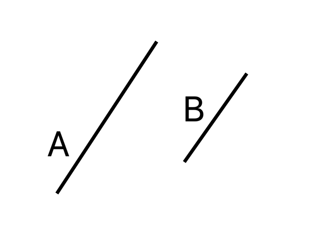
Are they parallel? “Of course, at least very nearly so” you may think. How do you know? “Just look!” If you wanted to be more careful, you might try drawing a line, as straight as you can make it, that intersects both A and B and using a protractor to measure the resulting angles. I will grant your ability to measure these angles, which are local measurements, but how do you know the line you drew is straight?
The problem of saying whether two line segments are parallel is equivalent to the problem of comparing two vectors (the tangent vectors to the line segments, in this case) at different points. The set of tangent vectors at one point is a vector space; the set of tangent vectors at another point is another vector space. These two vector spaces are like worlds unto themselves. How do we compare a vector in one space to a vector in another?
What you’re used to doing is looking at the vector’s components. Thus at point A, I can introduce two basis vectors, \(\vec{e}_1\) and \(\vec{e}_2\). (You may be used to seeing \(\vec{e}_x\) and \(\vec{e}_y\), or \(\hat{x}\) and \(\hat{y}\), or \(\hat{i}\) and \(\hat{j}\).) Then vector \(\vec{v}\) at A can be decomposed as \(\vec{v} = v^1 \vec{e}_1 + v^2\vec{e}_2\), where \(v^1\) and \(v^2\) are two numbers. Similarly vector \(\vec{u}\) at B can be decomposed as \(\vec{u} = u^1\vec{e}_1 + u^2\vec{e}_2\). Can I just compare the components (\(v^1\),\(v^2\)) and (\(u^1\),\(u^2\))? Alas, no. If we try, we’re immediately faced with the same problem. How do we know that \(\vec{e}_1\) at A is the same as \(\vec{e}_1\) at B? This is no idle worry. Even in flat space, radial and angular polar coordinate basis vectors point in different directions at different points.
If only we could pick up a vector at A and move it to B without changing the vector in transit, then we could do the comparison locally at B. One can imagine physically picking up an arrow and trying to move it without rotating it. How can I be sure it has experienced no torque? And isn’t it odd that a physics question just popped up in what should be something purely mathematical?
By the way, the “draw a straight line and use a protractor” strategy runs into the same problem. A “straight line” just means a line whose tangent vector doesn’t change as one moves along it. So to identify a line straight, we must be able to compare vectors at different locations.
What is needed is a connection—a rule for translating vectors. Let’s show this with a simple illustration. Say we stick with 2D and only interest ourselves in the direction of vectors. A fanciful but perfectly adequate way of quantifying direction would be to lay down a small analog clock at each point in space. The hour number the vector points at is its direction. It plays exactly the role of basis vectors. Then we might want to compare the direction of vectors at two points by comparing the numbers they point at, and from comparing vectors at nearby points, we could define a derivative of the vector. The worry is, what if the clock numbers are rotated with respect to each other? Then this comparison will be wrong:

Now, my connection is a rule that tells me how much I must rotate clock numbers to compare vectors at two points. E.g. to compare {\vec v} at A and at B, “move v at A to B” by taking the value at A and then rotating its value back by two hours to “translate” it to B. Now that the “translated” vector is at B, one can compare it to the vector already at B by subtracting the numbers they point to on the clock. Now we see that they point to the same number, so they are the same vector.
It is clear that the connection depends greatly on my choice of basis vectors, of how I orient those clocks. Is that all there is to it? A necessary (and, it turns out, sufficient) condition is that what \(\vec{v}\) is when moved from A to B should not depend on the path I take when moving \(\vec{v}\). If it does depend on the path, then the idea of a unique value of \(\vec{v}\) from A at B loses its meaning.
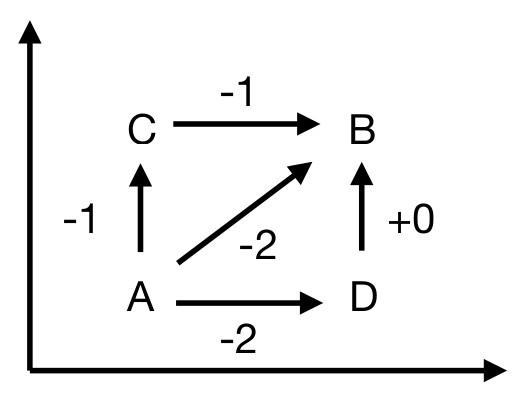
The connection I drew at the four segments above had this property, that A\(\rightarrow\)C\(\rightarrow\)B gives the same result as A\(\rightarrow\)D\(\rightarrow\)B. That’s because I derived that connection explicitly from clock rotations. However, let us now change our perspective. Let us think of the connection as an object in its own right. (No longer imagine that there are clocks embedded in flat space, where you could see by eye whether they were rotated with respect to each other.) Call the connection \(\tilde{A}\). At each point, it tells you how rapidly the 12 o’clock direction rotates as one moves in any direction. Say these numbers can be anything. Then the reqirement of path-independence is a very strict condition. Most values of \(\tilde{A}\) on those segments will not give this property. For example:
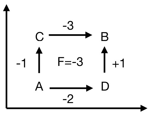
Note that if I start at A and move my vector on a closed circuit A\(\rightarrow\)C\(\rightarrow\)B\(\rightarrow\)D\(\rightarrow\)A, my vector is different when it returns to its starting point! This is the signature of curvature in my space.
What should my connection be? What should the corresponding curvature be? Pure logic, pure mathematics will not tell you; anything is logically, mathematically possible. This means it is an empirical question. We must do an experiment to find the curvature. And the curvature presumably came to have the value it does because it is a physical field with its own dynamics which we physicists can hope to discover.
In general relativity, what we call gravity is actually the manifestation of spacetime curvature. Whereas in Newtonian theory, we say that planets orbit the sun rather than traveling on straight lines because of a force of gravity, in relativity we say that there is no force acting on the planets, and they are traveling on straight lines, but they’re traveling on straight lines in a spacetime slightly curved by the influence of the sun.
You might balk at the idea that a “slight” curvature can do this. Surely an ellipse is more than slightly different from a straight line? Here it is important to remember that it is not space that is curved but spacetime. It is the worldline of a planet as it moves through 4D spacetime, moving “up” in time while spiraling in space, that is only slightly different from what we would consider a straight line in flat (Minkowski) spacetime. Here’s the picture:
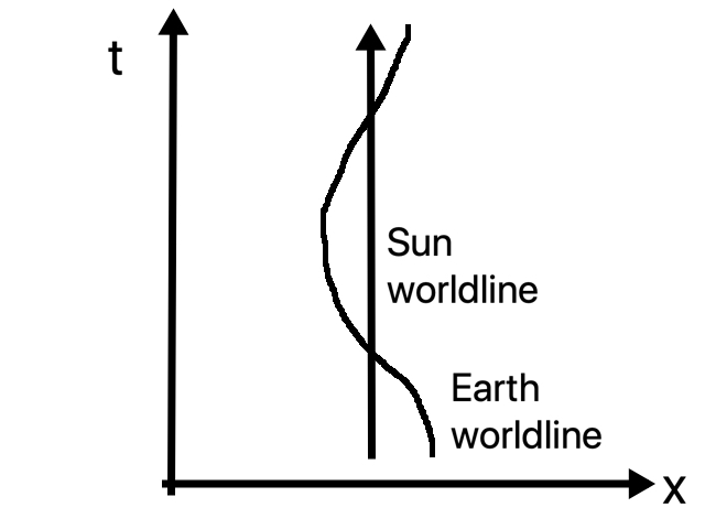
So, what we call free-fall is actually (if GR is right) inertial motion; its how a body with zero acceleration moves. A surprising consequence of this is that a person standing still on the surface of the Earth has nonzero acceleration because that person is not in free fall! In Newtonian physics, we would say that the acceleration is zero because two forces (normal force and gravity) cancel each other; in relativity, we say that the acceleration is nonzero because of the one and only acting force (the normal force from the ground).
That’s general relativity, but in modern physics all fundamental forces appear as curvatures associated with connections. For example, suppose I have two real scalar fields living in my spacetime, \(\phi_1\) and \(\phi_2\), which are non-interacting and identical in every way. There is clearly a symmetry in this problem. Suppose at one moment in time, \(\phi_1\) is a gaussian centered on point A while \(\phi_2\) is a gaussian centered on point B. Now, I tell you to close your eyes, and while you’re not looking, I instantaneously swap the two fields, so now \(\phi_1\) is centered at B and \(\phi_2\) is centered at A. When you open your eyes, you will not know that anything has changed. Because the fields are identical, no experiment could show a difference. This is an indication that, really, nothing has changed—I just relabeled the fields.
It is, in fact, more convenient to group my two real fields together into a single complex scalar field \(\phi = \phi_1 + i \phi_2 = \left|\phi\right| e^{i\psi}\). Then my relabeling amounts to a global change of phase \(\psi\). Wave phases in themselves are physically meaningless—only phase differences are meaningful and show up as interference effects.
As was the case with basis vectors, there’s no reason my phase convention can’t vary from point to point. It just means that when taking spatial derivatives of my field to solve the wave equation, I must use a covariant derivative, one that uses a connection to take into account how the meaning of \(\phi_1\) and \(\phi_2\) (or, equivalently, of \(\psi\)) changes from point to point.
The situation is, in fact, exactly that illustrated above with the different clocks at each point. Once we have defined our connection, we needn’t force it to have zero curvature. We can give the connection its own dynamics, subject to the spacetime and phase symmetries of the problem. In its most natural dynamics, the connection \(\tilde{A}\) can be identified as the electromagnetic vector potential, its curvature \(F\) as the field strength tensor (i.e. the electric and magnetic fields), and its evolution equations correspond to Maxwell’s equations. The effect of local phase redefinitions (“rotating the clocks with respect to each other”) on the connection is what we recognize as a gauge transformation of the vector potential. What we initially thought of as two real scalar fields turns out to be a single charged scalar field.
In undergraduate physics, one starts from the electric and magnetic fields. Then one introduces the vector potential as a mathematical trick for calculating these fields. Finally, one notices that a whole equivalence class of \(\tilde{A}\) fields give the same \(\vec{E}\) and \(\vec{B}\) fields, i.e. that there is a gauge freedom. Since \(\tilde{A}\) is considered just a tool, all these \(\tilde{A}\)s are considered to be physically equivalent.
In graduate physics, the line of thinking is exactly reversed. One starts with a local symmetry. The one we considered was the simplest: \(\phi_1\) and \(\phi_2\) can be rotated into each other in any way that preserves \(\phi_1^2 + \phi_2^2\). One can imagine more complicated possibilities. If there were 3 fields and the symmetry is that one can rotate them into each other in any way that preserves \(\phi_1^2+\phi_2^2+\phi_3^2\), there would be three independent ways of rotating into each other (for example, mixing \(\phi_1\) and \(\phi_2\), or mixing \(\phi_2\) and \(\phi_3\), or mixing \(\phi_1\) and \(\phi_3\)). Each would have its own connection. So, one starts with the set (actually, the group, in the precise mathematical term) of symmetry transformations. These dictate the connection’s gauge transformation. Finally, one computes the curvature corresponding to this connection(s), which is the equivalent of the \(\vec{E}\) and \(\vec{B}\) fields.
What to expect when beginning research
I think you will find that the greatest challenges to early success in research are not intellectual but psychological.
Before seriously beginning research, a student’s main experience with physics problem-solving is homework. A homework set will contain a few unrelated problems; it will be due about a week after it is handed out. When a student sits down to work on a homework assignment, he or she may reasonably expect the gratification of finishing in a few hours. If the student has worked for a couple of hours on one problem and made no progress on it, just one dead end after another, this would be a sign of something wrong; probably the student doesn’t understand the material well enough and should go to office hours before proceeding.
Research works on a very different timescale. A research project often takes one to two years to get publishable results, and longer stretches are not uncommon. Most of your time will be spent on dead ends before you hit on something that works. On any given morning, you will go into your office or lab, work on your project for a full day, and when you go home for supper, the project will not be in a significantly different state than when you came to work. This is not what you are used to, and there is a danger that you will fall into one of two reactions. First, you may become discouraged and depressed; you may find it difficult to continue exerting your full effort when the results seem so modest. Second, you may become complacent. Since it is not disconcerting for a day to go without progress, you may not worry when weeks or months go by without progress. That, however, is a problem and a sign that something about the project or your approach to it should be reassessed.
Your advisor has gotten used to this and will be a help here. He or she will help you learn to split up your multi-year project into tiny steps, so that you can have a reasonable-sized goal for what you will do the next day or the next week. Soon enough, you will learn to do this yourself. If you’re like me, you’ll keep a planner, write down goals for a day, and get a great deal of satisfaction from putting checkmarks next to them. Your advisor will also have learned from hard experience that weeks spent on dead ends, although unavoidable (after all, it wouldn’t be research if people already knew the results and how to get them), do add up and eventually become a problem. You want to learn to fail quickly, to recognize as soon as possible when something isn’t going to work, so you should be somewhat impatient to have a check of whether your idea can work before filling in all of the details.
We wish PhD students to move as quickly as possible to the forefront of research in some area. The fastest way to do that is to specialize to some very specific problem of current interest, so that is what we do. It’s probably the best thing, but it does have the disadvantage of making PhD students narrow in their knowledge and competence. A mark of your growing scientific maturity is how you begin to broaden yourself as you approach your dissertation. Indeed, if all goes well, this process continues at the postdoc and professor levels. It is something you must largely direct yourself, and it will often feel like you must sacrifice immediate research productivity to do it. In the hour you spend at a colloquium, you could indeed have gotten more done in the lab, but in the long run it will be better for your development as a scientist to go to the colloquium anyway. Consider also the astronomy lunch program and the AMO journal club, where you can discuss recent scientific developments with students and faculty. Naturally, your broadening efforts will always be a secondary priority after your research project, but it is important to keep expending a bit of time and effort toward it week after week, year after year.